Figure 6: Early AD Library5 sample structure

Overview

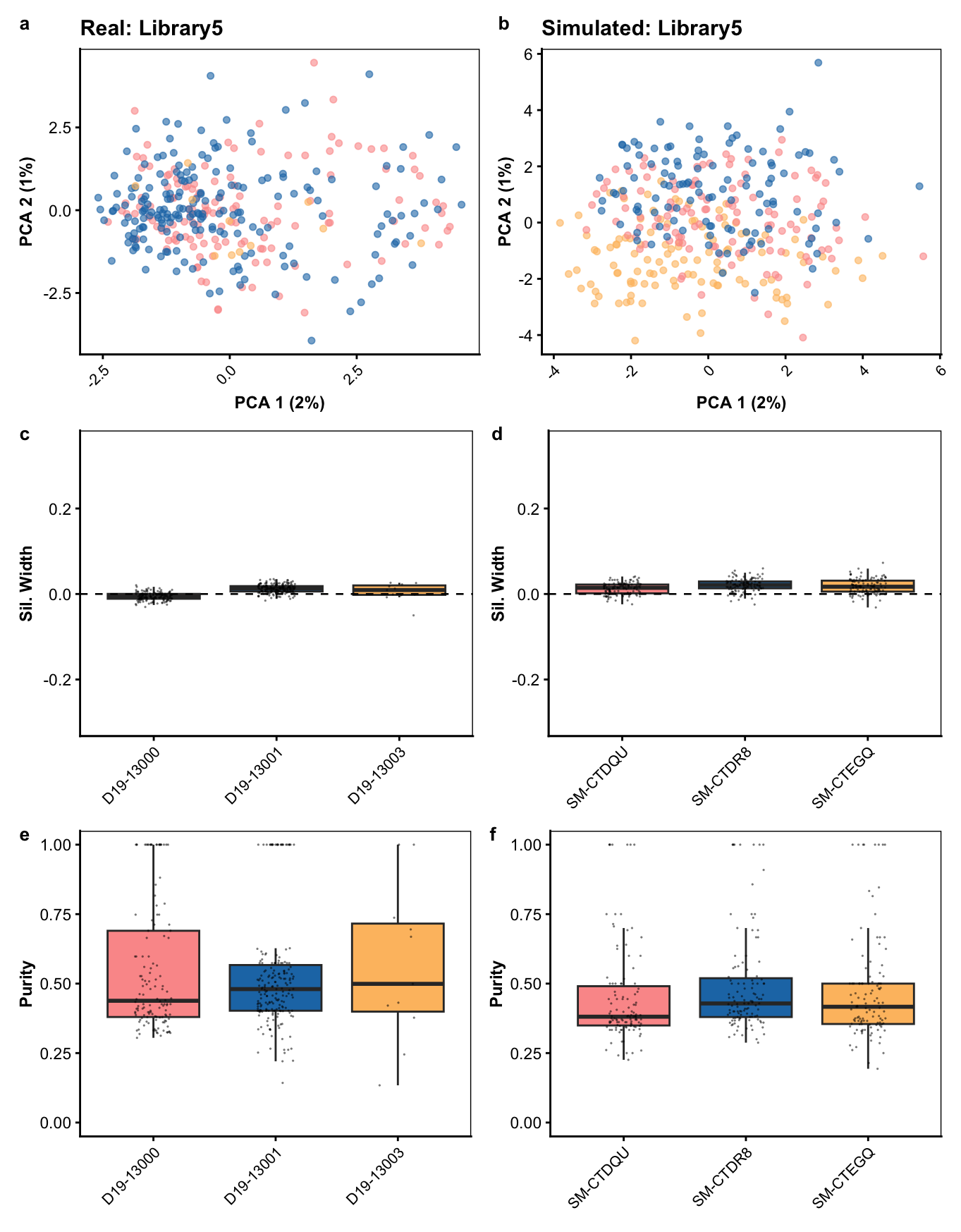
This document reproduces the early AD Library5 panel for manuscript Figure 6 from the SingleCellExperiment objects provided with this repository.\ The figure compares real and simulated cells using PCA, silhouette width, and neighbor purity, with sample colors mapped independently by sample order so that corresponding real and simulated sample groups use the same colors.

All inputs used below are stored in data/Figure6/SCEs.

Load Library5 Data

Show code

real_sces <- readRDS("data/Figure6/SCEs/batch_subsets_real.rds")
sim_sces <- readRDS("data/Figure6/SCEs/sim_results.rds")

sce_real <- real_sces[["Library5"]]
sce_sim <- sim_sces[["Library5"]]

Process Data

Show code

sce_real <- logNormCounts(sce_real)
sce_real <- runPCA(sce_real)

sce_sim <- logNormCounts(sce_sim)
sce_sim <- runPCA(sce_sim)

sil_real <- approxSilhouette(reducedDim(sce_real, "PCA"), sce_real$Sample)
sil_sim <- approxSilhouette(reducedDim(sce_sim, "PCA"), sce_sim$Sample)

pure_real <- neighborPurity(reducedDim(sce_real, "PCA"), sce_real$Sample)
pure_sim <- neighborPurity(reducedDim(sce_sim, "PCA"), sce_sim$Sample)

Plot Settings

Show code

kelly_colors <- c(
  "#FB9A99", "#1F78B4", "#FDBF6F", "#E31A1C", "#33A02C",
  "#FF7F00", "#6A3D9A", "#B15928", "#A6CEE3", "#B2DF8A",
  "#CAB2D6", "#191919", "#00C5CD", "#7FFF00", "#FF1493",
  "#FFD700", "#0000FF", "#8B4513", "#006400", "#4682B4"
)

real_samples <- sort(unique(sce_real$Sample))
sim_samples <- sort(unique(sce_sim$Sample))

real_color_map <- setNames(kelly_colors[seq_along(real_samples)], real_samples)
sim_color_map <- setNames(kelly_colors[seq_along(sim_samples)], sim_samples)
library_color_map <- c(real_color_map, sim_color_map)

pub_theme <- theme_cowplot(font_size = 10) +
  theme(
    axis.text.x = element_text(angle = 45, hjust = 1, size = 8),
    axis.title = element_text(size = 9, face = "bold"),
    legend.position = "none",
    panel.border = element_rect(colour = "black", fill = NA, linewidth = 0.5)
  )

make_metric_plot <- function(df, y_val, y_lab, ylims, is_silhouette = FALSE) {
  p <- ggplot(df, aes(x = factor(Cluster), y = .data[[y_val]], fill = factor(Cluster))) +
    geom_boxplot(outlier.shape = NA, alpha = 1, linewidth = 0.5) +
    geom_jitter(width = 0.15, size = 0.4, alpha = 0.5, color = "black", stroke = 0.1) +
    scale_fill_manual(values = library_color_map) +
    labs(x = NULL, y = y_lab) +
    coord_cartesian(ylim = ylims) +
    pub_theme

  if (is_silhouette) {
    p <- p + geom_hline(yintercept = 0, linetype = "dashed", color = "black")
  }

  p
}

Early AD Library5 Figure

Show code

p_pca_real <- suppressMessages(
  plotPCA(sce_real, colour_by = "Sample") +
    scale_color_manual(values = library_color_map) +
    labs(title = "Real: Library5") +
    pub_theme
)

p_pca_sim <- suppressMessages(
  plotPCA(sce_sim, colour_by = "Sample") +
    scale_color_manual(values = library_color_map) +
    labs(title = "Simulated: Library5") +
    pub_theme
)

p_sil_real <- make_metric_plot(
  data.frame(V = sil_real$width, Cluster = sce_real$Sample),
  "V",
  "Sil. Width",
  c(-0.30, 0.35),
  TRUE
)

p_sil_sim <- make_metric_plot(
  data.frame(V = sil_sim$width, Cluster = sce_sim$Sample),
  "V",
  "Sil. Width",
  c(-0.30, 0.35),
  TRUE
)

p_pure_real <- make_metric_plot(
  data.frame(V = pure_real$purity, Cluster = sce_real$Sample),
  "V",
  "Purity",
  c(0, 1)
)

p_pure_sim <- make_metric_plot(
  data.frame(V = pure_sim$purity, Cluster = sce_sim$Sample),
  "V",
  "Purity",
  c(0, 1)
)

figure6_library5 <- (p_pca_real | p_pca_sim) /
  (p_sil_real | p_sil_sim) /
  (p_pure_real | p_pure_sim) +
  plot_annotation(
    tag_levels = "a",
    theme = theme(plot.tag = element_text(face = "bold"))
  )

figure6_library5