Figure 4: Quantitative benchmarking summary

Overview

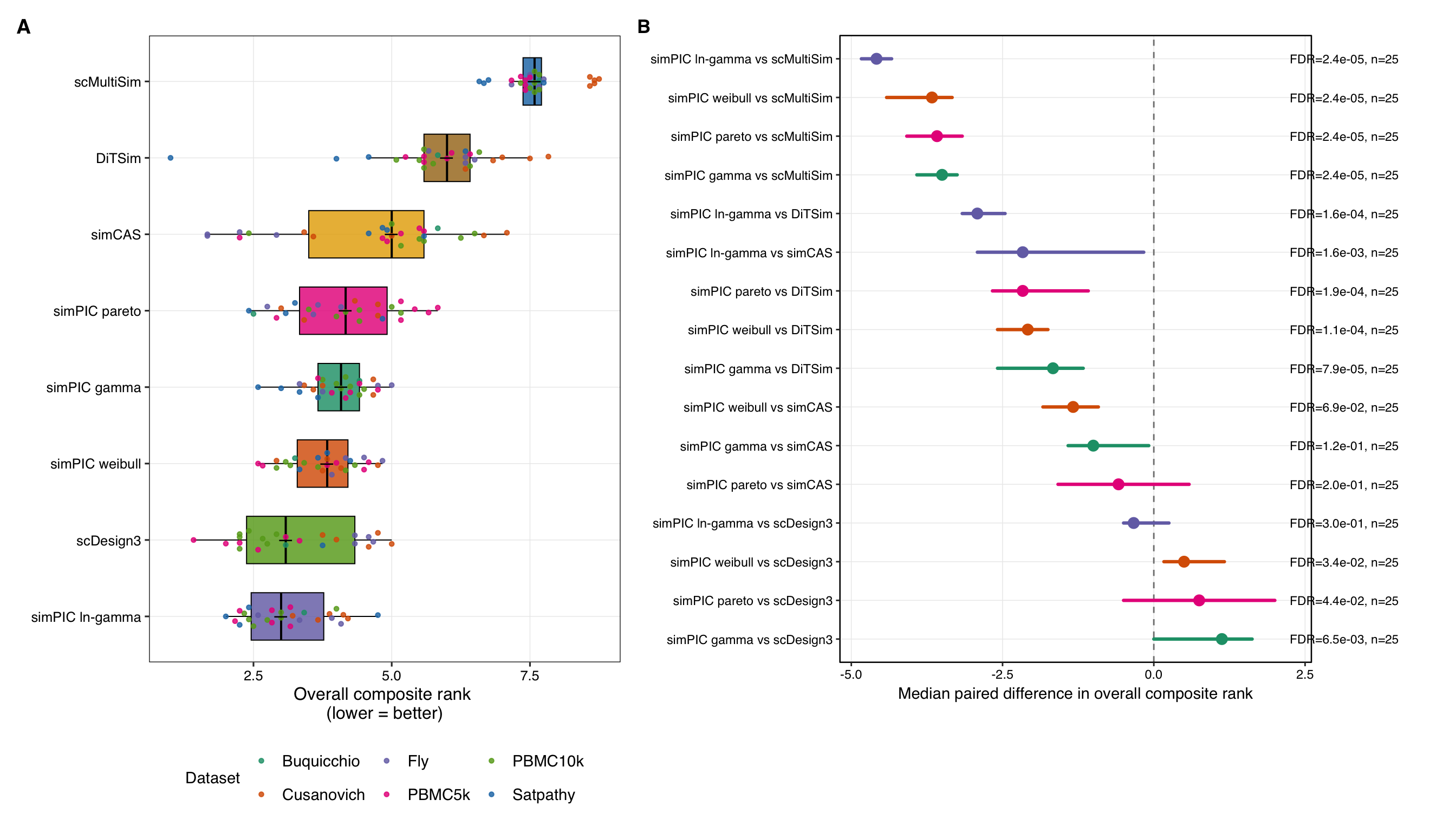
This document reproduces the manuscript Figure 4 panels from the processed benchmarking tables provided with this repository. Panel A summarizes overall simulator performance across cell types using the overall composite rank, where lower ranks indicate better agreement with real data. Panel B shows paired comparisons between each simPIC variant and competing methods on matched cell types.

All inputs used below are stored in data/Figure4.

Load Data

Show code

overall_composite <- read_csv(
  "data/Figure4/overall_composite_rank.csv",
  show_col_types = FALSE
)

paired_results <- read_csv(
  "data/Figure4/panelB_paired_results.csv",
  show_col_types = FALSE
)

Plot Settings

Show code

all_methods_order <- c(
  "simPIC-weibull",
  "simPIC-gamma",
  "simPIC-ln-gamma",
  "simPIC-pareto",
  "scDesign3",
  "simCAS",
  "DiTSim",
  "scMultiSim"
)

ds_levels <- c(
  "Buquicchio",
  "Cusanovich",
  "Fly",
  "PBMC5k",
  "PBMC10k",
  "Satpathy"
)

pretty_method_labels <- c(
  "simPIC-weibull" = "simPIC weibull",
  "simPIC-gamma" = "simPIC gamma",
  "simPIC-ln-gamma" = "simPIC ln-gamma",
  "simPIC-pareto" = "simPIC pareto",
  "scDesign3" = "scDesign3",
  "simCAS" = "simCAS",
  "DiTSim" = "DiTSim",
  "scMultiSim" = "scMultiSim"
)

tool_colours <- c(
  "simPIC-weibull" = "#D95F02",
  "simPIC-gamma" = "#1B9E77",
  "simPIC-ln-gamma" = "#7570B3",
  "simPIC-pareto" = "#E7298A",
  "scDesign3" = "#66A61E",
  "simCAS" = "#E6AB02",
  "DiTSim" = "#A6761D",
  "scMultiSim" = "#1F78B4"
)

dataset_colours <- c(
  "Buquicchio" = "#1B9E77",
  "Cusanovich" = "#D95F02",
  "Fly" = "#7570B3",
  "PBMC5k" = "#E7298A",
  "PBMC10k" = "#66A61E",
  "Satpathy" = "#1F78B4"
)

theme_pub <- function(base_size = 11) {
  theme_bw(base_size = base_size, base_family = "Helvetica") +
    theme(
      panel.grid.major = element_line(colour = "grey92", linewidth = 0.25),
      panel.grid.minor = element_blank(),
      panel.border = element_rect(colour = "black", fill = NA, linewidth = 0.45),
      axis.text = element_text(colour = "black"),
      axis.title = element_text(colour = "black"),
      plot.tag = element_text(face = "bold", size = base_size + 2),
      plot.margin = margin(6, 6, 6, 6),
      legend.title = element_text(size = base_size - 1),
      legend.text = element_text(size = base_size - 1)
    )
}

Panel A

Show code

panelA_df <- overall_composite |>
  mutate(
    method = factor(method, levels = all_methods_order),
    dataset = factor(dataset, levels = ds_levels)
  ) |>
  group_by(method) |>
  mutate(method_median = median(overall_composite_rank, na.rm = TRUE)) |>
  ungroup() |>
  mutate(method = fct_reorder(method, method_median, .desc = FALSE))

pA <- ggplot(panelA_df, aes(x = overall_composite_rank, y = method)) +
  geom_boxplot(
    aes(fill = method),
    width = 0.62,
    outlier.shape = NA,
    alpha = 0.82,
    linewidth = 0.35,
    color = "black"
  ) +
  geom_quasirandom(
    aes(color = dataset),
    width = 0.16,
    size = 1.15,
    alpha = 0.82,
    varwidth = FALSE
  ) +
  stat_summary(
    fun = median,
    geom = "point",
    shape = 95,
    size = 5,
    color = "black"
  ) +
  scale_fill_manual(values = tool_colours[names(tool_colours) %in% levels(panelA_df$method)]) +
  scale_color_manual(values = dataset_colours, name = "Dataset") +
  scale_y_discrete(labels = pretty_method_labels) +
  guides(fill = "none") +
  labs(
    tag = "A",
    x = "Overall composite rank \n(lower = better)",
    y = NULL
  ) +
  theme_pub(base_size = 12) +
  theme(legend.position = "bottom")

Panel B

Show code

paired_results <- paired_results |>
  arrange(median_diff) |>
  mutate(comparison = factor(comparison, levels = rev(comparison)))

x_text <- max(
  c(paired_results$ci_high, paired_results$median_diff),
  na.rm = TRUE
) + 0.25

pB <- ggplot(paired_results, aes(x = median_diff, y = comparison, color = simPIC_method)) +
  geom_vline(xintercept = 0, linetype = 2, color = "grey50", linewidth = 0.5) +
  geom_segment(
    aes(x = ci_low, xend = ci_high, yend = comparison),
    linewidth = 1.1,
    lineend = "round"
  ) +
  geom_point(size = 3.2) +
  geom_text(
    aes(
      x = x_text,
      label = paste0(
        "FDR=",
        ifelse(is.na(padj), "NA", formatC(padj, format = "e", digits = 1)),
        ", n=",
        n_celltypes
      )
    ),
    hjust = 0,
    size = 3,
    color = "black"
  ) +
  scale_color_manual(
    values = tool_colours[
      names(tool_colours) %in% unique(as.character(paired_results$simPIC_method))
    ]
  ) +
  labs(
    tag = "B",
    x = "Median paired difference in overall composite rank",
    y = NULL
  ) +
  coord_cartesian(clip = "off") +
  theme_pub(base_size = 11) +
  theme(
    legend.position = "none",
    plot.margin = margin(5.5, 95, 5.5, 5.5)
  )

Combined Manuscript Figure

Show code

wrap_plots(pA, pB, ncol = 2) +
  plot_annotation(
    theme = theme(
      plot.tag = element_text(face = "bold", size = 14),
      plot.tag.position = c(0, 1)
    )
  )