Figure 3: Key characteristic comparison

Overview

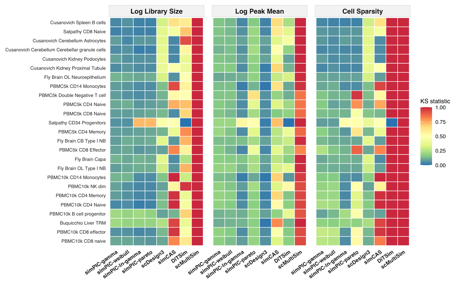
This document reproduces the manuscript Figure 3 panels from the processed data provided with this repository. The first panel shows key distributional characteristics for one example cell type, Cusanovich Kidney Podocytes, comparing the real data with simulated outputs. The second panel summarizes KS statistics across selected cell types and metrics.

All inputs used below are stored in data/Figure3. The code prints the plots in the knitted document and does not save any figures or intermediate files.

Show code

data_dir <- "data/Figure3"
panel_stat <- "KS"
target_cell_type <- "Cusanovich_Kidney_Podocytes"
metrics_main <- c("library_size", "peak_mean", "cell_sparsity")

tool_dirs <- c(
  "simPIC_gamma" = file.path(data_dir, "simPIC_gamma"),
  "simPIC_weibull" = file.path(data_dir, "simPIC_weibull"),
  "simPIC_lngamma" = file.path(data_dir, "simPIC_lngamma"),
  "simPIC_pareto" = file.path(data_dir, "simPIC_pareto"),
  "scDesign3" = file.path(data_dir, "scDesign3"),
  "simCAS" = file.path(data_dir, "simCAS"),
  "DiTSim" = file.path(data_dir, "DiTSim"),
  "scMultiSim" = file.path(data_dir, "scMultiSim")
)

real_dir <- file.path(data_dir, "Real")

focus_order <- c(
  "Real", "simPIC_gamma", "simPIC_weibull", "simPIC_lngamma",
  "simPIC_pareto", "scDesign3", "simCAS"
)

extract_matrix <- function(obj) {
  if (inherits(obj, "SingleCellExperiment")) {
    if ("counts" %in% assayNames(obj)) {
      return(as(counts(obj), "dgCMatrix"))
    }
    return(as(assay(obj, 1), "dgCMatrix"))
  }

  if (inherits(obj, "SummarizedExperiment")) {
    return(as(assay(obj, 1), "dgCMatrix"))
  }

  if (inherits(obj, c("dgCMatrix", "dgTMatrix", "Matrix"))) {
    return(as(obj, "dgCMatrix"))
  }

  if (is.matrix(obj)) {
    return(as(obj, "dgCMatrix"))
  }

  if (is.list(obj)) {
    for (nm in c("counts", "count", "matrix", "mat")) {
      if (!is.null(obj[[nm]])) {
        return(as(obj[[nm]], "dgCMatrix"))
      }
    }
  }

  stop("Cannot extract count matrix from: ", paste(class(obj), collapse = ", "))
}

compute_stats <- function(mat) {
  np <- nrow(mat)
  list(
    library_size = log1p(Matrix::colSums(mat)),
    peak_mean = log1p(Matrix::rowMeans(mat)),
    cell_sparsity = 1 - Matrix::colSums(mat > 0) / np
  )
}

calc_wasserstein_1d <- function(x, y, n_grid = 2000) {
  x <- x[is.finite(x)]
  y <- y[is.finite(y)]
  if (length(x) == 0 || length(y) == 0) {
    return(NA_real_)
  }

  probs <- seq(0, 1, length.out = n_grid)
  qx <- quantile(x, probs = probs, names = FALSE, type = 8, na.rm = TRUE)
  qy <- quantile(y, probs = probs, names = FALSE, type = 8, na.rm = TRUE)
  mean(abs(qx - qy))
}

build_file_index <- function(dir_path) {
  if (dir.exists(dir_path)) {
    files <- list.files(
      dir_path,
      pattern = "\\.rds$",
      ignore.case = TRUE,
      full.names = TRUE
    )
  } else {
    files <- list.files(
      dirname(dir_path),
      pattern = paste0("^", basename(dir_path), ".*\\.rds$"),
      ignore.case = TRUE,
      full.names = TRUE
    )
  }

  if (length(files) == 0) {
    return(tibble(
      file_path = character(),
      base = character(),
      base_lower = character()
    ))
  }

  tibble(
    file_path = files,
    base = tools::file_path_sans_ext(basename(files)),
    base_lower = tolower(base)
  )
}

find_indexed_file <- function(file_index, cell_type) {
  if (nrow(file_index) == 0) {
    return(NULL)
  }

  idx <- which(file_index$base == cell_type)
  if (length(idx) == 0) {
    idx <- which(file_index$base_lower == tolower(cell_type))
  }
  if (length(idx) == 0) {
    idx <- grep(tolower(cell_type), file_index$base_lower, fixed = TRUE)
  }
  if (length(idx) == 0) {
    return(NULL)
  }

  file_index$file_path[idx[1]]
}

load_sce_from_index <- function(file_index, cell_type) {
  fp <- find_indexed_file(file_index, cell_type)
  if (is.null(fp)) {
    return(NULL)
  }

  obj <- tryCatch(
    readRDS(fp),
    error = function(e) {
      warning("Could not read ", basename(fp), ": ", conditionMessage(e))
      NULL
    }
  )
  if (is.null(obj)) {
    return(NULL)
  }

  mat <- extract_matrix(obj)
  if (ncol(mat) > nrow(mat) * 5) {
    mat <- t(mat)
  }
  as(mat, "dgCMatrix")
}

tool_palette <- c(
  "Real" = "#111111",
  "simPIC_gamma" = "#1B9E77",
  "simPIC_weibull" = "#D95F02",
  "simPIC_lngamma" = "#7570B3",
  "simPIC_pareto" = "#E7298A",
  "scDesign3" = "#66A61E",
  "simCAS" = "#E6AB02",
  "DiTSim" = "#A6761D",
  "scMultiSim" = "#1F78B4"
)

metric_labels <- c(
  library_size = "Log Library Size",
  peak_mean = "Log Peak Mean",
  cell_sparsity = "Cell Sparsity"
)

x_labels <- c(
  "Real" = "Real",
  "simPIC_gamma" = "simPIC\ngamma",
  "simPIC_weibull" = "simPIC\nweibull",
  "simPIC_lngamma" = "simPIC\nln-gamma",
  "simPIC_pareto" = "simPIC\npareto",
  "scDesign3" = "scDesign3",
  "simCAS" = "simCAS",
  "DiTSim" = "DiTSim",
  "scMultiSim" = "scMultiSim"
)

pub_theme <- theme_bw(base_size = 11, base_family = "Helvetica") +
  theme(
    panel.grid.major = element_line(colour = "grey94", linewidth = 0.3),
    panel.grid.minor = element_blank(),
    panel.border = element_rect(colour = "black", linewidth = 0.5),
    axis.title.x = element_text(size = 9, colour = "black", margin = margin(t = 6)),
    axis.title.y = element_text(size = 9, colour = "black", margin = margin(r = 6)),
    axis.text.y = element_text(size = 8, colour = "black"),
    axis.ticks = element_line(colour = "black", linewidth = 0.3),
    legend.position = "none",
    plot.title = element_text(face = "bold", size = 9.5, hjust = 0.5),
    plot.margin = margin(8, 4, 4, 4)
  )

make_violin_panel <- function(metric, stats_list, stat_df, present_names, panel_stat = "KS") {
  dat <- lapply(present_names, function(nm) {
    tibble(tool = nm, value = stats_list[[nm]][[metric]])
  }) |>
    bind_rows() |>
    mutate(tool = factor(tool, levels = present_names))

  stat_sub <- stat_df |>
    filter(.data$metric == .env$metric)

  y_range <- range(dat$value, na.rm = TRUE)
  y_span <- diff(y_range)
  if (y_span == 0) {
    y_span <- 1
  }

  value_col <- if (panel_stat == "KS") "ks" else "wasserstein"
  y_upper <- y_range[2] + y_span * 0.22
  y_lab <- y_range[2] + y_span * 0.10

  if (metric == "peak_mean" && "scMultiSim" %in% dat$tool) {
    scmultisim_max <- max(dat$value[dat$tool == "scMultiSim"], na.rm = TRUE)
    y_upper <- 0.25 * scmultisim_max
    y_lab <- y_upper * 0.98
  }

  label_df <- stat_sub |>
    mutate(
      tool = factor(tool, levels = present_names),
      y = y_lab,
      label = if (panel_stat == "KS") {
        sprintf("%.2f", .data[[value_col]])
      } else {
        sprintf("WS=%.3f", .data[[value_col]])
      }
    )

  ggplot(dat, aes(x = tool, y = value, fill = tool, colour = tool)) +
    geom_violin(trim = TRUE, scale = "width", linewidth = 0.4, alpha = 0.82) +
    geom_text(
      data = label_df,
      aes(x = tool, y = y, label = label),
      colour = "black",
      size = 2.2,
      fontface = "bold",
      vjust = 0
    ) +
    scale_fill_manual(values = tool_palette[present_names]) +
    scale_colour_manual(values = tool_palette[present_names]) +
    scale_x_discrete(labels = x_labels[present_names]) +
    coord_cartesian(ylim = c(y_range[1] - y_span * 0.05, y_upper)) +
    labs(title = metric_labels[metric], x = NULL, y = metric_labels[metric]) +
    pub_theme +
    theme(
      axis.text.x = element_text(
        size = 8,
        face = "bold",
        angle = 35,
        hjust = 1,
        lineheight = 0.8
      )
    )
}

make_density_panel <- function(metric, stats_list, present_names) {
  df <- lapply(present_names, function(nm) {
    tibble(dataset = nm, value = stats_list[[nm]][[metric]])
  }) |>
    bind_rows() |>
    filter(is.finite(value)) |>
    mutate(dataset = factor(dataset, levels = present_names))

  ggplot(df, aes(x = value, colour = dataset, fill = dataset)) +
    geom_density(alpha = 0.15, linewidth = 0.8, adjust = 1.2) +
    scale_colour_manual(values = tool_palette[present_names], name = NULL) +
    scale_fill_manual(values = tool_palette[present_names], name = NULL) +
    scale_y_sqrt() +
    labs(x = metric_labels[metric], y = "Density") +
    pub_theme
}

make_density_difference_panel <- function(metric, stats_list, present_names, n_grid = 512) {
  real_vals <- stats_list[["Real"]][[metric]]
  real_vals <- real_vals[is.finite(real_vals)]

  all_vals <- unlist(
    lapply(present_names, function(nm) stats_list[[nm]][[metric]]),
    use.names = FALSE
  )
  all_vals <- all_vals[is.finite(all_vals)]

  xr <- range(all_vals, na.rm = TRUE)
  x_grid <- seq(xr[1], xr[2], length.out = n_grid)
  dens_real <- density(real_vals, from = xr[1], to = xr[2], n = n_grid, na.rm = TRUE)

  diff_df <- lapply(setdiff(present_names, "Real"), function(nm) {
    vals <- stats_list[[nm]][[metric]]
    vals <- vals[is.finite(vals)]
    dens_tool <- density(vals, from = xr[1], to = xr[2], n = n_grid, na.rm = TRUE)
    tibble(dataset = nm, x = x_grid, diff = dens_tool$y - dens_real$y)
  }) |>
    bind_rows() |>
    mutate(dataset = factor(dataset, levels = setdiff(present_names, "Real")))

  ggplot(diff_df, aes(x = x, y = diff, colour = dataset, fill = dataset)) +
    geom_hline(yintercept = 0, colour = "grey55", linewidth = 0.4) +
    geom_area(alpha = 0.18, position = "identity") +
    geom_line(linewidth = 0.8) +
    scale_colour_manual(values = tool_palette[setdiff(present_names, "Real")], name = NULL) +
    scale_fill_manual(values = tool_palette[setdiff(present_names, "Real")], name = NULL) +
    coord_cartesian(
      ylim = quantile(diff_df$diff, probs = c(0.01, 0.99), na.rm = TRUE)
    ) +
    labs(
      x = paste0(metric_labels[metric], " (Density difference vs Real)"),
      y = "Density difference"
    ) +
    pub_theme
}

process_cell_type <- function(target_cell_type,
                              real_index,
                              tool_indices,
                              metrics_main,
                              focus_order,
                              panel_stat = "KS") {
  real_mat <- load_sce_from_index(real_index, target_cell_type)
  if (is.null(real_mat)) {
    warning("Real data not found for: ", target_cell_type)
    return(NULL)
  }

  sim_mats <- lapply(names(tool_indices), function(nm) {
    load_sce_from_index(tool_indices[[nm]], target_cell_type)
  })
  names(sim_mats) <- names(tool_indices)
  sim_mats <- Filter(Negate(is.null), sim_mats)

  present_tools <- names(sim_mats)
  if (length(present_tools) == 0) {
    warning("No simulated data found for: ", target_cell_type)
    return(NULL)
  }

  present_names <- c("Real", present_tools)
  focus_names <- intersect(focus_order, present_names)
  all_mats_ct <- c(list(Real = real_mat), sim_mats)
  stats_list_ct <- lapply(all_mats_ct, compute_stats)

  ks_ct <- lapply(metrics_main, function(met) {
    lapply(present_tools, function(tn) {
      x <- stats_list_ct[["Real"]][[met]]
      y <- stats_list_ct[[tn]][[met]]
      x <- x[is.finite(x)]
      y <- y[is.finite(y)]
      ks <- if (length(x) >= 2 && length(y) >= 2) {
        round(suppressWarnings(ks.test(x, y))$statistic, 2)
      } else {
        NA_real_
      }
      tibble(cell_type = target_cell_type, metric = met, tool = tn, ks = ks)
    }) |>
      bind_rows()
  }) |>
    bind_rows()

  wass_ct <- lapply(metrics_main, function(met) {
    lapply(present_tools, function(tn) {
      wd <- round(
        calc_wasserstein_1d(
          stats_list_ct[["Real"]][[met]],
          stats_list_ct[[tn]][[met]]
        ),
        4
      )
      tibble(cell_type = target_cell_type, metric = met, tool = tn, wasserstein = wd)
    }) |>
      bind_rows()
  }) |>
    bind_rows()

  stat_ct <- if (panel_stat == "KS") ks_ct else wass_ct

  violin_panels <- lapply(
    metrics_main,
    make_violin_panel,
    stats_list = stats_list_ct,
    stat_df = stat_ct,
    present_names = present_names,
    panel_stat = panel_stat
  )

  density_panels <- lapply(
    metrics_main,
    make_density_panel,
    stats_list = stats_list_ct,
    present_names = focus_names
  )

  density_diff_panels <- lapply(
    metrics_main,
    make_density_difference_panel,
    stats_list = stats_list_ct,
    present_names = focus_names
  )

  panel_abc <- wrap_plots(violin_panels, nrow = 1) +
    plot_annotation(tag_levels = "a")

  density_panels <- lapply(
    density_panels,
    function(panel) panel + theme(legend.position = "none")
  )

  density_diff_panels <- lapply(
    density_diff_panels,
    function(panel) panel + theme(legend.position = "none")
  )

  panel_density_main <- wrap_plots(density_panels, nrow = 1)
  panel_density_diff <- wrap_plots(density_diff_panels, nrow = 1)

  panel_abc / panel_density_main / panel_density_diff +
    plot_layout(heights = c(1, 1, 1)) +
    plot_annotation(
      title = target_cell_type,
      tag_levels = list(c("a", "b", "c", "d", "e", "f", "g", "h", "i"))
    )
}

real_index <- build_file_index(real_dir)
tool_indices <- lapply(tool_dirs, build_file_index)

podocytes_plot <- process_cell_type(
  target_cell_type = target_cell_type,
  real_index = real_index,
  tool_indices = tool_indices,
  metrics_main = metrics_main,
  focus_order = focus_order,
  panel_stat = panel_stat
)

podocytes_plot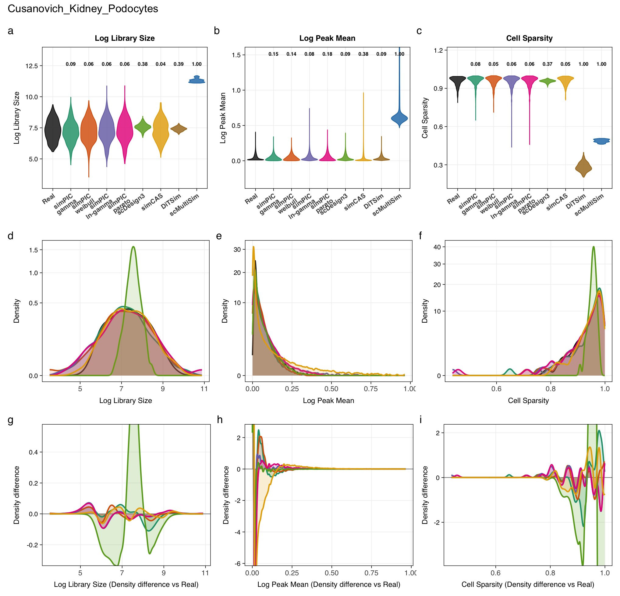

Figure 2 heatmap

Show code

metric_type <- "KS"

if (metric_type == "KS") {
  infile <- "data/Figure3/KS_all_selected_celltypes.csv"
  value_col <- "ks"
  legend_title <- "KS statistic"
} else {
  stop("metric_type must be 'KS' for this reproducible figure.")
}

dat <- read_csv(infile, show_col_types = FALSE)

plot_df <- dat |>
  filter(metric %in% c("library_size", "peak_mean", "cell_sparsity")) |>
  mutate(
    metric = recode(
      metric,
      library_size = "Log Library Size",
      peak_mean = "Log Peak Mean",
      cell_sparsity = "Cell Sparsity"
    ),
    metric = factor(
      metric,
      levels = c("Log Library Size", "Log Peak Mean", "Cell Sparsity")
    ),
    tool = factor(
      tool,
      levels = c(
        "simPIC_gamma",
        "simPIC_weibull",
        "simPIC_lngamma",
        "simPIC_pareto",
        "scDesign3",
        "simCAS",
        "DiTSim",
        "scMultiSim"
      )
    )
  ) |>
  filter(!is.na(.data[[value_col]]))

cell_order <- plot_df |>
  filter(tool == "simPIC_weibull") |>
  group_by(cell_type) |>
  summarise(score = mean(.data[[value_col]], na.rm = TRUE), .groups = "drop") |>
  arrange(score) |>
  pull(cell_type)

plot_df <- plot_df |>
  mutate(
    cell_type_label = gsub("_", " ", cell_type),
    cell_type_label = factor(
      cell_type_label,
      levels = rev(gsub("_", " ", cell_order))
    )
  )

tool_labels <- c(
  simPIC_gamma = "simPIC-gamma",
  simPIC_weibull = "simPIC-weibull",
  simPIC_lngamma = "simPIC-ln-gamma",
  simPIC_pareto = "simPIC-pareto",
  scDesign3 = "scDesign3",
  simCAS = "simCAS",
  DiTSim = "DiTSim",
  scMultiSim = "scMultiSim"
)

p <- ggplot(plot_df, aes(x = tool, y = cell_type_label, fill = .data[[value_col]])) +
  geom_tile(color = "white", linewidth = 0.35) +
  facet_grid(. ~ metric, scales = "free_x", space = "free_x") +
  scale_x_discrete(labels = tool_labels, drop = FALSE) +
  scale_fill_distiller(
    palette = "Spectral",
    name = legend_title
  ) +
  labs(x = NULL, y = NULL) +
  theme_minimal(base_size = 10, base_family = "Helvetica") +
  theme(
    panel.grid = element_blank(),
    axis.text.x = element_text(
      angle = 35,
      hjust = 1,
      vjust = 1,
      size = 8,
      colour = "grey15",
      face = "bold"
    ),
    axis.text.y = element_text(size = 7, colour = "grey20"),
    axis.title = element_blank(),
    strip.text = element_text(size = 10, face = "bold", colour = "grey10"),
    strip.background = element_rect(
      fill = "grey96",
      colour = "grey85",
      linewidth = 0.4
    ),
    panel.spacing.x = unit(4, "mm"),
    legend.position = "right",
    legend.title = element_text(size = 9),
    legend.text = element_text(size = 8),
    plot.margin = margin(8, 8, 8, 8)
  )

p